Getting Started

Use this page to get acquainted with Alpha Trading Labs. This will be helpful as a reference to guide you in setting up your model as well as writing a valuation function for a model. If you have never used Alpha Trading Labs before, go through the entirety of this document, otherwise skip to the section which you need.

• Tutorial
  • Getting Aquainted
  • Understanding the Model
  • Create Multiple Models at Once
  • Save and Find Your Models
• What the Results Summary Means
• Model Parameters
• Trading Column Parameters
• Valuation Functions
• Why Use Hold

Tutorial

This tutorial is a quick guide on how to create and test a model on Alpha Trading Labs. You will of course need an account and need to be signed into the site.

• Click on “New Startegy” on the top left to get started.

Getting Aquainted

• You will be met with the main editing page of for your model, it should look something like this:

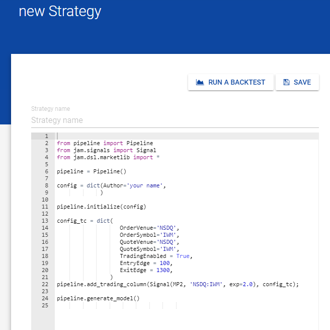
• The code you see is the default set up for a working model. We will now test it so you can start to get a feel on how the site works.
• First thing you will want to do is name your strategy, you can do this by clicking on “Startegy Name”
  • for this tutorial you can simply use “Tutorial”

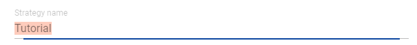
• Now click on “SAVE”, you should see a green box on the top right highlighting that you have saved your startegy.
  • Note: as you edit your model it should auto save however it is always a good habit to manually save after any edit

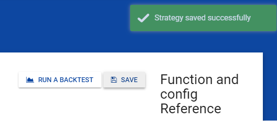
• Lets test the default model, click on “RUN A BACKTEST” next to the save button
• You should be met with a window that looks like this:

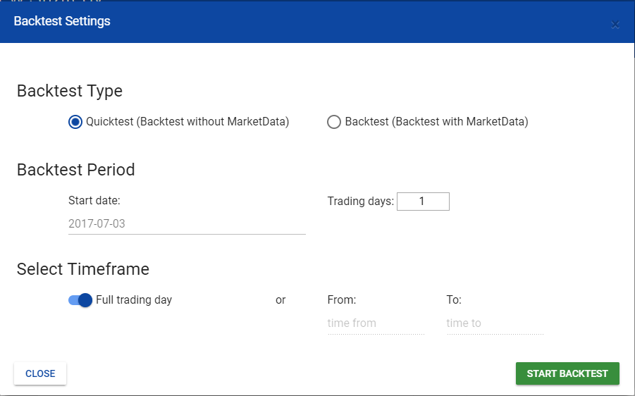
• Choose whether you want to do a “Quicktest” or “Backtest”
  • Quicktest will not use market data but will execute quicker
  • Backtest will use market data but will take longer
  • Note: If you Backtest you can only do 1 day
• For the tutorial leave “Quicktest”
• Set you Backtest Period
  • Choose the start date
  • Choose the number of days to run the test starting from the start date
• For the tutorial we will leave the default date and 1 trading day
• Select a Timeframe
  • Depending on your model you may not want to test a full trading day. You can set the times between 9.30am to 4.00pm EST in which you want to run your test
• For the tutorial we will leave “full trading day” selected
• Click on “START BACKTEST”
• Wait for the model to run
• After a few seconds you should be met with a screen similar to this:

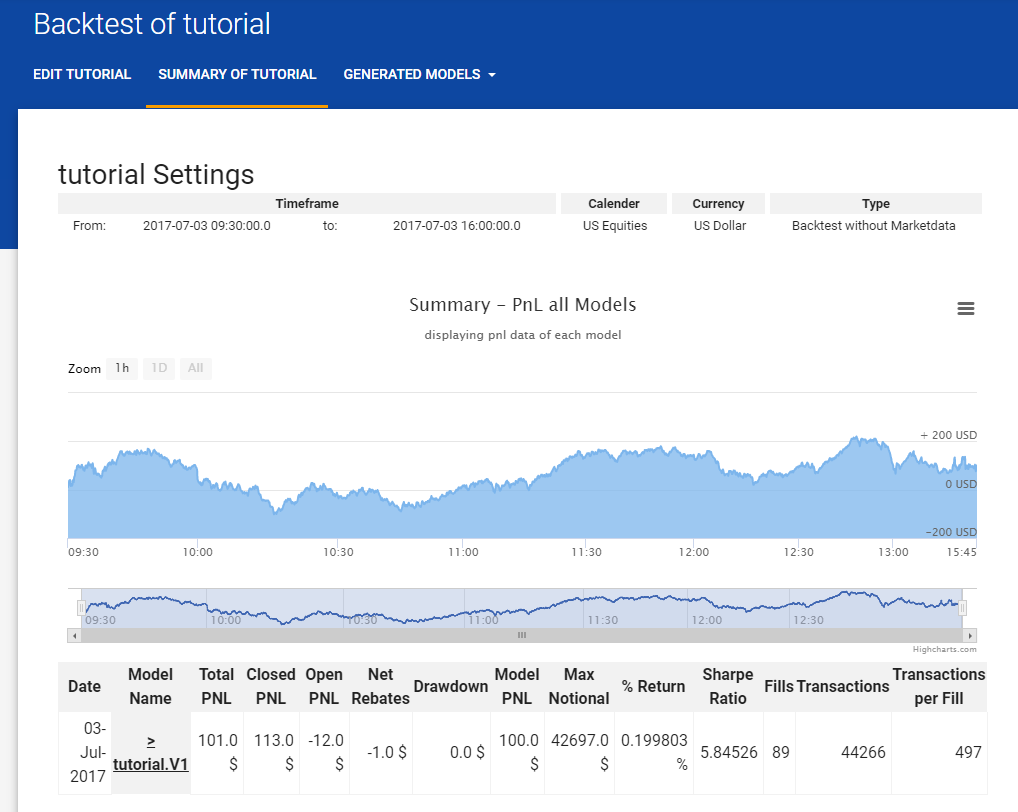
• These are the results from running the model
  • For more information on what the results mean go to What the Results Summary Means
• This summary should tell you whether or not your model is successful

Understanding the Model

Now that you are familiar with the how to maneuver the basics of the site let’s look at the model, how it is structured and what each part means

• The model is has four basic parts to it

1. The first is the imports and initialization, highlighted here:

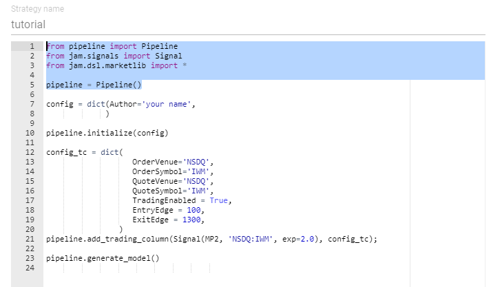
• These lines are necessary to create and run the model, you should leave these lines as there are
  • Pipeline sets up your model and its parameters
  • Signal evaluates the given valuation function
  • marketlib is a library of helper and valuation function you can use ( Marketlib )

2. The next part consists of setting up the model parameters, highlighted here:

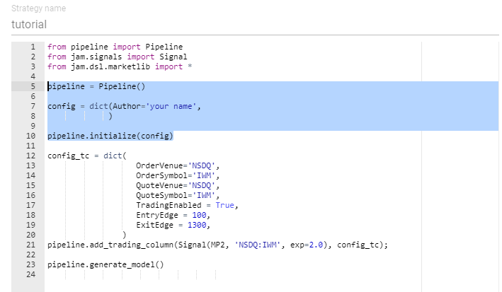
• Here you can set up your model by overriding the default parameters, in order for the model to meet your needs
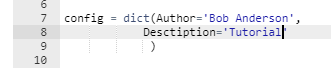
  • for example set yourself as the author:

• Go to Model Parameters to see all the parameters you can set and what they mean

3. The third part consists of the trading column parameters, highlighted here:

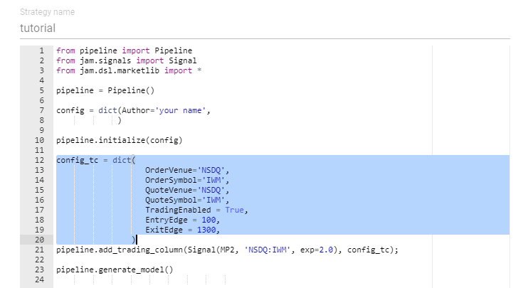
• These parameters are very important as they will determine important factors in your trading model such as
  • What security symbol to trade
  • Order size
  • Trading strategies
  • And many more
  • For example, change the security symbol you want to trade:

• To see all the parameters you can change in your trading column see Trading Column Parameters
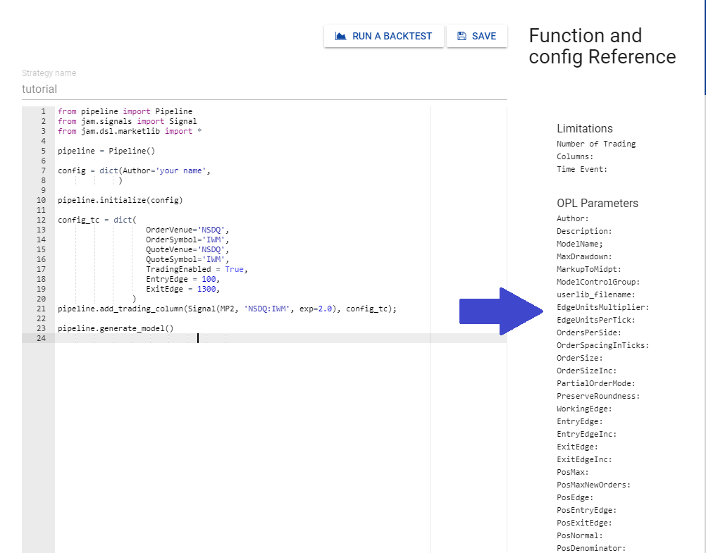
• You can also see all the parameters and what they do on the right hand side of the editing view:

4. Finally you have the part that actually creates your model, highlighted here:

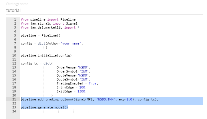
• The most important part of this, what is inside of Signal() is the only thing you should change from these two lines

  • Signal interprets your valuation function as such:

    Signal(valuation Function, *arguments valuation function takes)

  • By default the model uses MP2 a valuation function included in Marketlib, where “NSDQ:IWM” and exp=2 are the arguments being passed into MP2

• Now you can write your own valuation function and replace MP2 with it, passing whatever arguments your function might take.

  • For example, lets use MP2 (the defualt valuation function already passed in Signal). If we were to have written this valuation function ourselves we could put it in the model like this:

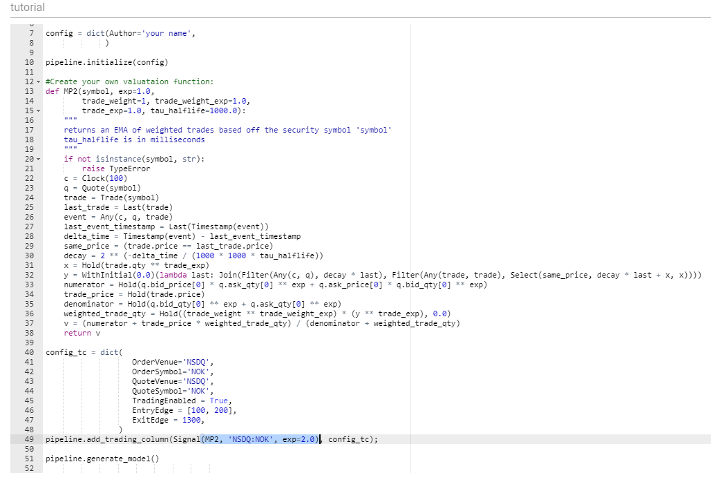
• Again, make sure to update Signal with your new valuation function and its arguments.
  • In this case since were still using MP2 there is no need to change it
• For more information on writing your own valuation function and understanding how the DSL can help you write a function such as MP2 see Valuation Functions

Create Multiple Models at Once

Now that you know the basics about how the model works here is an additional trick to help you create multiple models using the same valuation function but with different parameters.

• Go to the trading column parameters for any given parameter add a second value in the form of a list like this:

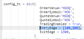
• This will create two models where one has the EntryEdge set to 100 and the second to 200, and all the other paramters remain the same.

  • you can do this with all parameters at the same time, where the first element in the list of the given parameters will be the value for the first model, the second values in the lists for the second model etc.
  • the number of models generated will be equal to the length of the longest list of arguments in a given parameter
  • Note: don’t add too many arguments, where it would be wise to keep it to 2 arguments

• For this tutorial we will keep it simple and only add a second argument to “EntryEdge”

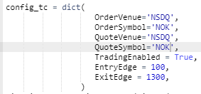
  • Note: we kept the changed Order and Quite symbol ‘NOK’
  • If you run the model with NOK don’t forget to also change Signal to:

  Signal(MP2, ‘NSDQQ:NOK’, exp=2.0)

• Same as before click “RUN BACKTEST” and set up your test

  • Again we will keep all the default values for this tutorial

• You should now see something similar to this:

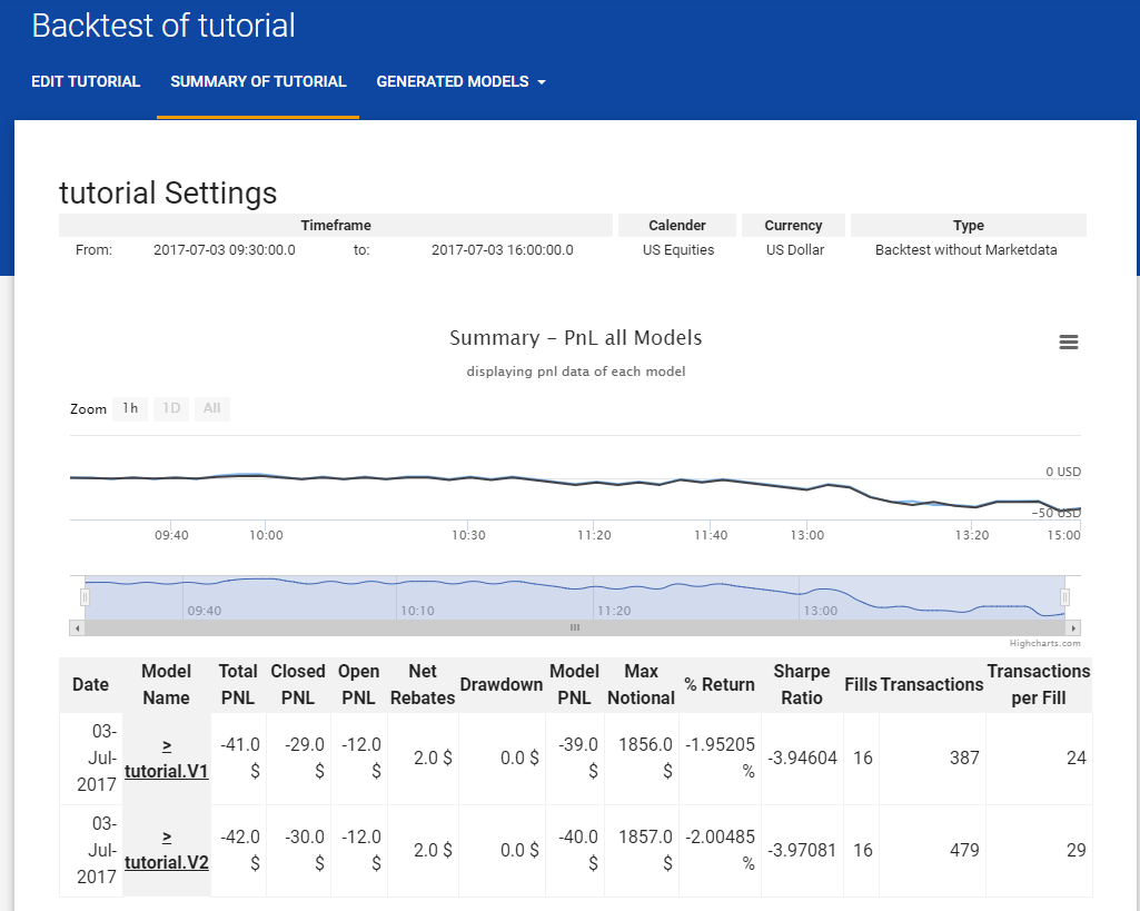
• As you can see there are now two sets of results which you can compare side by side
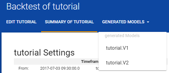
• You can also see them individually and with more details if you go to the “GENERATED MODELS” tab on top:

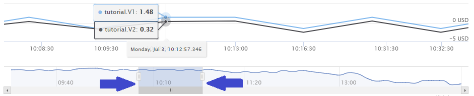
• The graph may look like a single graph if the models are similar but it is actually displaying both models
• you zoom into a the graph by reducing the timeframe
• Full graph:

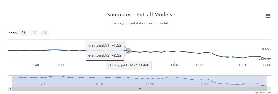
• Zoomed Graph, where you can now see the difference between the two models:

Use your own Valuation Function

Now that you know how to change the parameters, whenever you are ready to write and use your own valuation function

Save and Find Your Models

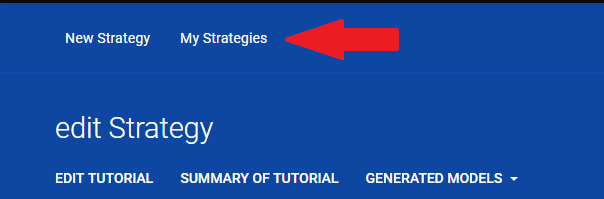
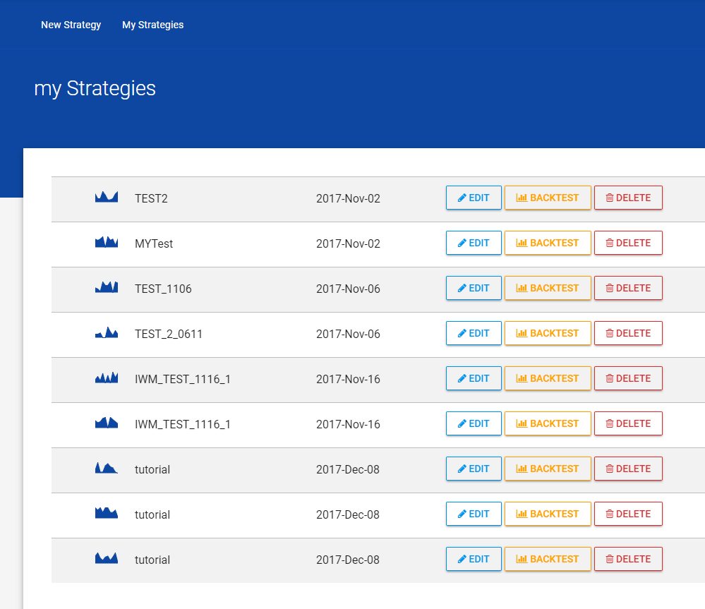
• You can now find your saved strategies, as well as any generated models created from running a backtest, on the “My Strategies” tab on top:

• As you can see there are three “tutorial” models to click here, the first one being the one we generated with all the default parameters, and the other two are the generated models from when we rant the multiple parameters in one go:

You should now be familiar with how to navigate the application and how to create a model. You are now ready to create your own strategies and write your own valuation function. Use the more detailed information below as well as the information on Alpha Trading Labs DSL and Marketlib

What the Results Summary Means

Here is a brief summary of what all the results actually mean:

Result	Definition
Total PNL	total Profit or Loss (open + closed)
Closed PNL	amount sold (profit or loss on closed positions)
Open PNL	amount of profit or loss of still open positions at the time model ended
Net Rebates	Trading Rebates - Trading Fees
Drawdown	Difference between the last peak and the ending price of the security
Model PNL	Total profit or loss of the model (Total PNL + Net Rebates)
Max Notional	How much was invested on the model
% Return	% return of investments (Model PNL / Max Notional)
Sharpe Ratio	Volatility of the model
Fills	Total executed buy and sell orders
Transactions	Total requested transactions
Transactions per Fills	Transactions / Fills

Model Parameters

Here are the model parameters you can change:

self.config = dict(
      Author = 'Author Unknown',
      Description = 'No Description',
      ModelName='Unknown',
      MaxDrawdown = 65000,
      MarkupToMidpt = True,
      ModelControlGroup = 'AlphaLabs | Test | |',
      userlib_filename = '',
        )

• Author: Your name as “Firstname Lastname”
• Description: Description of the model, what you want it to achieve and how.
• Model Name: Name of your model.
• Max Drawdown: TO BE IMPLEMENTED, do not change D=Maximum loss your model can have. This is an integer value in dollar amount. When the model drawdown value reaches this limit, the model will be moved to exit mode. In exit mode, if the net position of the model is zero, it will cancel all the outstanding orders. This parameter is not used while back testing the model.
• Markup To Midpoint: TO BE IMPLEMENTED, do not change
• Model Control Group: TO BE IMPLEMENTED, do not change
• User Library Filename: TO BE IMPLEMENTED, do not change The absolute path to your library file containing your personally defined algorithms.

Trading Column Parameters

Here are the Trading Column Parameters that you can manipulate in order for your model to behave in the way that you want it to.

self.config_tc = dict(
      EdgeUnitsMultiplier=100,
      EdgeUnitsPerTick=1000,
      OrdersPerSide=3,
      OrderSpacing=1,
      OrderSpacingInTicks = True,
      MinOrderSize = 1,
      OrderSize = 100,
      OrderSizeInc = 100,
      PartialOrderMode = 'FULL',
      PreserveRoundness = False,
      WorkingEdge = 50,
      PosMax = 300,
      PosMaxNewOrders = 300,
      PosNormal = 300,
      EntryEdge = 100,
      EntryEdgeInc = 10,
      ExitEdge = 200,
      ExitEdgeInc = 20,
      PosEntryEdge = 0,
      PosExitEdge = 0,
      PosEdge = 200,
      EntryRoundingMode = 1,
      ExitRoundingMode = 0,
      ExitColumnMode = 3,
      PortfolioPosEdge = 0,
      PortfolioPosDenominator = 0,
      PortfolioBeta = 1.0,
      AddingOrderType = 'ALO',
      MaxEdge = 50000,
      MaxPriceImprovement = -1,
      MinJoinVolume = 100,
      OrderDelay = 0,
      MinOrderHitTake = 500,
      RemovalEntryEdge = 100,
      RemovalExitEdge = 100,
      RemovalOrderType = 'IOC',
      CancelDelay = 0,
      PairBeta = 1.0,
      PairDenom = 100,
      PairEdge = 100,
      BidsOnly = False,
      AsksOnly = False,
      PairColumnType = 0,
      Strategy = '2 Sided Market Making',
      TradingEnabled = True,
      OrderVenue='NSDQ',
      OrderSymbol='GRPN',
      QuoteVenue='NSDQ',
      QuoteSymbol='GRPN',
      PairVenue='NSDQ',
      PairSymbol='GRPN',
       )

• Edge Unit Multiplier” This parameter is used to convert the stock price in decimal to an integer value. If the price of the security is represented in 2 decimals (for example as $123.45), the edge unit multiplier should be set to 100. The default value of this parameter should be 100

• Edge Units Per Tick: EdgeUnitsPerTick indicates number of units we want to have per tick. For example if a stock price ticks by $0.01, we would need edge unit multiplier as 100. And for the same stock, if the valuation function is expected to return a valuation price in milli pennies such as $123.45678, then EdgeUnitsPerTick should be set to 1000.

• Order Per Side: The parameter OrdersPerSide is used to set the maximum number of orders a trading column can place on a bid side and/or on offer side. However only one order can be placed on one price level. Valid values for this parameters are from 1 to 5

• Order Spacing: TO BE IMPLEMENTED, do not change

• Order Spacing In Ticks: TO BE IMPLEMENTED, do not change

• Min Order Size: TO BE IMPLEMENTED, do not change

• Order Size: Indicates minimum size of an order.

• Order Size Inc: TO BE IMPLEMENTED, do not change Default value of this parameter should be 100. This parameter is used to manually increase the order size through a GUI control.

• Partial Order Mode: TO BE IMPLEMENTED, do not change default value of this parameter is “FULL”.

• Preserve Roundness: TO BE IMPLEMENTED, do not change default value of this parameter is False.

• Working Edge: WorkingEdge is used while calculating bid and offer price. This will be added to ask price to get the good ask price. And will subtracted from bid price to get a good bid price. It is used both while entering and exiting a position.

• Pos Max: This parameter PosMax indicated the maximum position a trading column can have.

• Pos Max New Orders: TO BE IMPLEMENTED, do not change

• Pos Normal: This parameter would contain a value between 0 and PosMax. PosEntryEdge, PosExitEdge, and PosEdge parameter values will be applied in full after the position reaches the value set for this parameter. Until the total position reaches this PosNormal value, PosEntryEdge, PosExitEdge and PosEdge will be applied in proportion to the position.

• Entry Edge: EntryEdge is applied to bid and ask price while entering a position.

• Entry Edge Inc: TO BE IMPLEMENTED, do not change Default value of this parameter should be 10. This parameter is used to manually increase the EntryEdge value through a GUI control.

• Exit Edge: ExitEdge is applied to bid and ask price while exiting a position.

• Exit Edge Inc: TO BE IMPLEMENTED, do not change Default value of this parameter should be 10. This parameter is used to manually increase the ExitEdge value through a GUI control.

• Pos Entry Edge: PosEntryEdge is applied to bid and ask price while entering a position. PosEntryEdge will be added proportionately based on the position that has been acquired.

• Pos Exit Edge: PosExitEdge is applied to bid and ask price while exiting a position. Similar to PosEntryEdge, PosExitEdge will be added proportionately based on the position that has been acquired.

• Pos Edge: PosEdge is similar to WorkingEdge and is used while calculating bid and offer price. This will be added to ask price to get the good ask price. And will subtracted from bid price to get a good bid price. It is used both while entering and exiting a position and proportionately based on the poistion acquired.

• Entry Rounding Mode and Exit Rounding Mode: EntryRoundingMode and ExitRoundingMode can contain one of the following four values 0 – PRESERVE 1 = ADD, 2 = REDUCE 3 = DONT_ROUND, Valid values for EntryRoundingMode is 0, 1, and 3. And Valid values for ExitRoundingMode is 0, 1, 2, 3 EntryRoundingMode and ExitRoundingMode work together as a pair. Default value of EntryRoundingMode is 1 and ExitRoundingMode is 0.

  Example: Assume book contains following quantity on the bid and offer side (100 100 — 100 100) If a sell of 70 partially fills bid side leaving 30 residual, the book will look as follows (100 100 — 30 100) Now, if the rounding mode is set as follows

  1. EntryRoundingMode = 0, & ExitRoundingMode = 0 (PRESERVE_PRESERVE), No Orders will be placed, the book will look as follows (100 100 — 30 100)
  2. EntryRoundingMode = 1, & ExitRoundingMode = 0 (ADD_PRESERVE), An order will be sent to replenish the Bid side, the book will look as follows (100 100 — 30+100 100)
  3. EntryRoundingMode = 1, & ExitRoundingMode = 2 (ADD_REDUCE), An order will be sent to replenish the Bid side and reduce the Offer side by 30, the book will look as follows (100 70 — 30+100 100)
  4. EntryRoundingMode = 0, & ExitRoundingMode = 2 (PRESERVE_REDUCE), An order will be sent to reduce the Offer side by 30, the book will look as follows (100 70 — 30 100)
  5. EntryRoundingMode = 0, & ExitRoundingMode = 3 (PRESERVE_ADD), An order will be sent to replenish the Offer side, the book will look as follows (100 100+70 — 30 100)
  6. EntryRoundingMode = 3, & ExitRoundingMode = 3 (ADD_ADD), An order will be sent to replenish the Bid and Offer side, the book will look as follows (100 100+70 — 30+100 100)

• Exit Column Mode: ExitColumnMode is used while Hedging. Valid values for ExitColumnMode are 0, 1, and 2. Below are the description of each value 0 = None, 1 = INSIDE_ONLY, 2 = ALL_LEVELS, The Value 0 disables exit column mode, 1 means the order will only place on the inside level (level 0) and 2 means orders will be placed on all price levels.

• Portfolio Pos Edge: TO BE IMPLEMENTED, do not change default value of this parameter is 0.

• Portfolio Pos Denominator: TO BE IMPLEMENTED, do not change default value of this parameter is 0.

• Portfolio Beta: !!!!! TO BE IMPLEMENTED, do not change default value of this parameter is 1.0.

• Adding Order Type: AddingOrderType specifies the type of the Order that the trading column would create. Valid values for this parameter are ‘ALO’ (Add Liquidity Only), ‘LIMIT’, and ‘MARKET’.

• Max Edge: MaxEdge indicates maximum effective value for entry and exit edges. If the effective entry/exit edge reaches MaxEdge and the net position is greater than zero, then the orders will be canceled.

• Max Price Imporvement: MaxPriceImprovement is used to determine the bid and ask price. If MaxPriceImprovement is set to 0, then the trading column will join the best bid/offer price, regardless of how much the valuation price is through the book. If MaxPriceImprovement is greater than 0, then the trading column will be allowed to cross the best bid/offer price by MaxPriceImprovement times the EdgeUnitsPerTick. If MaxPriceImprovement is set to -1 (or less than 0), then MaxPriceImprovement feature will be disabled, the bid and ask price will be allowed to cross the best bid and offer regardless how far it is through the book.

• Min Join Volume: TO BE IMPLEMENTED, do not change Default value for this parameter is 100.

• Order Delay: TO BE IMPLEMENTED, do not change Default value for this parameter is 0.

• Min Order Hit rate: TO BE IMPLEMENTED, do not change Default value for this parameter is 500. This was originally used with removal price but not used any more.

• Removal Entry Edge: TO BE IMPLEMENTED, do not change The default value of this parameter is 100.

• Removal Exit Edge: TO BE IMPLEMENTED, do not change The default value of this parameter is 100.

• Removal Order Type: TO BE IMPLEMENTED, do not change The default value of this parameter is ‘IOC’.

• Cancel Delay: TO BE IMPLEMENTED, do not change Default value for this parameter is 0.

• Pair Beta: PairBeta is used by Pair Trading Column. It provides hedge ratio. The ratio is positive is the pair is directly proportional to this trading column. Default value of this parameter is 1.0

• Pair Denom: PairDenom is used by PairTradingColumn. This is used along with PairEdge. Effecive pair edge that the column calculates will be divided by this value before it gets applied.

• Pair Edge: PairEdge is used by PairTradingColumn. This is an additional edge during hedging.

• Bids Only: TO BE IMPLEMENTED, do not change Default value of this parameter is False.

• Asks Only: TO BE IMPLEMENTED, do not change Default value of this parameter is False.

• Pair Column Type: This parameter is used to specify the trading column type. Following are valid values for this parameter 0, 1, 2, 3, 4, and 5. Below are the description of each value. 0 = NON_PAIR, 1 = ENTER_LONG, 2 = ENTER_SHORT, 3 = EXIT_LONG, 4 = EXIT_SHORT, 5 = NON_PAIR_EXIT_ONLY Value 0 is used for creating TwoSidedMarketMaking trading column.

  • Value 1 is used by trading column specifically for entering long position. When PairBeta is greater than or equal to zero, LessLiquidBidAsk trading column will be created. When PairBeta is less than zero LessLiquidBidBid trading column will be created.
  • Value 2 is used by trading column for entering short position. When PairBeta is greater than or equal to zero, LessLiquidAskBid trading column will be created. When PairBeta is less than zero LessLiquidAskAsk trading column will be created.
  • Value 3 is used by trading column for exiting long position. When PairBeta is greater than or equal to zero, OfferHedgingBid trading column will be created. When PairBeta is less than zero OfferHedgingOffer trading column will be created.
  • Value 4 is used by trading column for exiting short position. When PairBeta is greater than or equal to zero, BidHedgingOffer trading column will be created. When PairBeta is less than zero BidHedgingBid trading column will be created.
  • Value 5 is used for creating a Non Pair Exit only trading column.

• Startegy: This is a string that provides a short description about the strategy. Used for administration purposes.

• Trading Enabled: Orders will be processed for this trading column only when this parameter is set to True. Default value of this parameter is True

• Order Venue: Order Venue and Order Symbol specifies the Exchange and Symbol for which this trading column will generate orders. OrderVenue should be configured as NSDQ for now.

• Order Symbol: Order Venue and Order Symbol specifies the Exchange and Symbol for which this trading column will generate orders. OrderVenue should be configured as NSDQ for now.

• Quote Venue: QuoteSymbol and QuoteVenue is the valuation symbol and the exchange providing this symbols market data. This is used for valuation.

• Quote Symbol: QuoteSymbol and QuoteVenue is the valuation symbol and the exchange providing this symbols market data. This is used for valuation.

• Pair Vanue and Pair Symbol: This is used in Pair Trading Column. It specifies Pair Venue and Pair Symbol while creating Spread Strategy.

Valuation Functions

Valuation Functions are the most important part of your model as they will dictate the price at which orders will be placed to buy and sell.

The model runs your valuation function continuously and extremely quickly in order to always have the correct price.

It is up to you to determine how you want that price to be calculated.

Write the valuation function using the DSL Alpha Trading Labs DSL which will enable you to access and manipulate real time market data on trades and quotes leading to an accurate price calculation.

• Note on how valuation functions work in the model: Valuation functions and the DSL work around Events nodes, mainly Trade and Quote where you will create a Trade and/or Quote variable for a given security symbol which will continuously update based on real market data. The valuation function is run continuously where certain lines of code will only run if in that ‘cycle’ of the valuation function the event that happened most recently is used in that line of code. To understand more about what this implies read through the rest of the MP2 example and Why Use Hold

MP2 is the valuation used by default on the application, we will go through the function to give you an idea about ways in which the DSL can be used. This should then allow you to create your own function which caters to whatever goal you want your model to achieve.

Note: Your valuation function can be just ass, less, or more complicated as MP2. It is up to you to determine what you want your valuation function to acomplish

Example Valuation Function MP2

MP2 returns an EMA (Exponential Moving Average) of weighted trades. What this means is the price it outputs is an average price which moves according to market data on trades, where more weight is given to the latest data. So if a lot of time goes by before a new trade happens then the value loses weight as the time passes, then when a new trade is registered the weight given to that data is much higher thus adjusting the price accordingly.

Throughout the example you will find links to items that are part of the Alpha Trading Labs DSL, read these in order to fully understand how MP2 works as a valuation function in the Alpha Trading Labs model

• italicized bullet points will serve as recommendations for when you write your valuation function

Here is the function as a whole where we will look in detail how it reaches the price output.

def MP2(symbol, exp=1.0,
              trade_weight=1, trade_weight_exp=1.0,
              trade_exp=1.0, tau_halflife=1000.0):

              """tau_halflife is in milliseconds"""

      if not isinstance(symbol, str):
              raise TypeError
      c = Clock(100)
      q = Quote(symbol)
      trade = Trade(symbol)
      event = Any(c, q, trade)
      last_trade = Last(trade)
      last_event_timestamp = Last(Timestamp(event))
      delta_time = Timestamp(event) - last_event_timestamp
      same_price = (trade.price == last_trade.price)
      decay = 2 ** (-delta_time / (1000 * 1000 * tau_halflife))
      x = Hold(trade.qty ** trade_exp)
      trade_price = Hold(trade.price)
      y = WithInitial(0.0)(lambda last: Join(Filter(Any(c, q), decay * last), Filter(Any(trade, trade), Select(same_price, decay * last + x, x))))
      numerator = Hold((q.bid_price[0] * (q.ask_qty[0] ** exp)) + (q.ask_price[0] * (q.bid_qty[0] ** exp)))
      denominator = Hold((q.bid_qty[0] ** exp) + (q.ask_qty[0] ** exp))
      weighted_trade_qty = Hold((trade_weight ** trade_weight_exp) * (y ** trade_exp))
      v = (numerator + (trade_price * weighted_trade_qty)) / (denominator + weighted_trade_qty)
      return v

MP2 looks at the trade data and creates a prices based of that data by assigning weight to it. In order to be able to change the calculated weight it has a series of arguments which can be changed, but are assigned a default value which will calculate prices with no extra weight. We will look at what each of these arguments do as they come up.

def MP2(symbol, exp=1.0,
              trade_weight=1, trade_weight_exp=1.0,
              trade_exp=1.0, tau_halflife=1000.0):

• It is a good idea to give your function a selection of arguments which can be changed, anything you may use as multipliers, exponents, decays, which you might want to alter later. This way you can easily change the way your model works by simply changing the arguments passed instead of writing a whole other function. Assign them default values as well so you do not have to define them every time.
• You will also want to include ‘symbol’ as an argument (always pass it the same symbol you set in your trading column parameters).

MP2 then initializes the Events it will keep track of during the time that the model runs:

if not isinstance(symbol, str):
              raise TypeError
      c = Clock(100)
      q = Quote(symbol)
      trade = Trade(symbol)
      event = Any(c, q, trade)

In this case, a Clock ‘c’ to keep track of a lack of events, Quote ‘q’ to have access to the book and any changes to it for the security symbol ‘symbol’ which you choose for your model, and Trade ‘trade’ to be able to see the latest actual trades for the security symbol. ‘event’ uses Any which will keep track of all three of these such that it is now possible to know which of the three events was the most recent to have happened.

• at the beggening of your valuation function you will want to set up all the events you want to use to calculate your price. Whether it be be only Quotes, Only Trades, or both like MP2 does.

These events all have properties which can help calculate a price. For example, you can set up variables using their attributes, which are important to your price calculation. MP2 sets up some variables which will be important to the EMA calculation:

last_trade = Last(trade)
same_price = (trade.price == last_trade.price)
last_event_timestamp = Last(Timestamp(event))
delta_time = Timestamp(event) - last_event_timestamp
decay = 2 ** (-delta_time / (1000 * 1000 * tau_halflife))
x = Hold(trade.qty ** trade_exp)
trade_price = Hold(trade.price)

MP2 keeps track of the Last trade that was executed, doing so in order to be able to calculate whether or not the price has changed since the last trade and the most recent trade (‘same_price’).

It keeps track of the change in time between the most recent event to have occurred and the one before it using Timestamp (‘delta_time’).

It sets up the decay value it will use later to determine the weight of values used in the final price calculation. It is clear that the higher delta_time is the bigger decay’s value will be. Notice: tau_halflife is used here to calculate decay, where default is 1000, but can be changed to either increase or decrease decay rate

It will Hold the weighted trade quantity Notice: weight of trade quantity is determined by trade_exp which can be changed and the default value is 1 meaning at default there is no extra weight attributed to quantity

Finally it will hold the trade price.

• you hold values for event attributes that will be used in calculations because it is possible that for any given ‘cycle’ in which the valuation function is run there might not be a new trade so for example trade.price would not execute that cycle, but by holding trade.price you ensure that you have available to you the most recent price in every ‘cycle’ of the valuation function to use in your calculation.

Now that the events and these values are set up we are ready to make the calculations

y = WithInitial(0.0)(lambda last: Join(Filter(Any(c, q), decay * last), Filter(Any(trade, trade), Select(same_price, decay * last + x, x))))
numerator = Hold((q.bid_price[0] * (q.ask_qty[0] ** exp)) + (q.ask_price[0] * (q.bid_qty[0] ** exp)))
denominator = Hold((q.bid_qty[0] ** exp) + (q.ask_qty[0] ** exp))
weighted_trade_qty = Hold((trade_weight ** trade_weight_exp) * (y ** trade_exp))
v = (numerator + (trade_price * weighted_trade_qty)) / (denominator + weighted_trade_qty)
return v

• These are some really good examples of how to use the :ref:`AL` in order to manipulate data.

We will look at these calculations line by line:

y = WithInitial(0.0)(lambda last: Join(Filter(Any(c, q), decay * last), Filter(Any(trade, trade), Select(same_price, decay * last + x, x))))

The first line is assigning to ‘y’ the calculated decayed trade quantity value. Doing so by using WithInitial Where it will assign 0.0 to ‘last’ where last in a sense holds the value for the next ‘cycle’. It then runs the anonymous lambda function proceeding it. (It is recommended to see the WithInitial documentation)

Within the lambda function we find a Join with two Filter arguments:

…Join(Filter(Any(c, q), decay * last), Filter(Any(trade, trade), Select(same_price, decay * last + x, x))))

the first filter will check if the Any is true, in other words if either c or q are the most recent events (remember c is the Clock and q is the Quote we initialized at the beginning), if they are then return decay * last (the value is assigned ‘last’ as well as ‘y’)

…Join(Filter(Any(c, q), decay * last)…

remember we created the value of decay before, so what this does is if there was no trade then decay the current value of last. For every continuous cycle where there is no trade the value of last is decayed more and more

• Using Any in this context as an argument for will check if any of the events passed as it’s arguments are the most recent event. You can think of it as returning True or False (although it’s not quite doing that, but we don’t need to worry about that)

The second filter also uses Any but notice it has trade twice, mainly because it requires two arguments. The purpose of this is that this filter will execute only if there has been a trade as the most recent event for this cycle of the valuation function. If that is the case then it will return the Select:

Filter(Any(trade, trade), Select(same_price, decay * last + x, x))))

What this select does is check if the value same_price (which we defined earlier) is true. * if true then return decay * last + x which is the decayed value of x plus the weighted trade quantity stored in x. * if false return x (the weighted trade quantity) The value is then assigned to ‘last’ to be stored and ‘y’ to be used

Select(same_price, decay * last + x, x)

So what this entire line does in essence is:

y = WithInitial(0.0)(lambda last: Join(Filter(Any(c, q), decay * last), Filter(Any(trade, trade), Select(same_price, decay * last + x, x))))

• when initialized returns the value 0.0 if no trade has happened yet.
• Once a trade happens for the first time it will return the weighted trade quantity x
• At that point onward if there is a new trade it will again return the weighted trade quantity
• if however there was no trade then the weighted trade quantity is decayed
• every continous cycle there is no new trade the weighted trade quantity is decayed further
• If there was a new trade event but the price did not change then the weighted trade quantity is decayed but the most recent weighted trade quantity is taken into account

This will allow to calculate the price using a weighted trade quantity which is decayed due to no new trades or changes in prices happening.

Now we calculate the first part of the numerator by cross multiplying and adding the bid price and ask quantity with ask price and bid quantity and hold the value, as such:

numerator = Hold((q.bid_price[0] * (q.ask_qty[0] ** exp)) + (q.ask_price[0] * (q.bid_qty[0] ** exp)))

The first part of the denominator will be calculates by adding weight to bid quantity with an exponent ‘exp’ (which is one of the function arguments, default is 1.0 so if you want more weight change this value) and adding that with the ask quantity also to the power of ‘exp’and hold it:

denominator = Hold((q.bid_qty[0] ** exp) + (q.ask_qty[0] ** exp))

Now we add more weight to our previously calculated weighted trade quantity ‘y’ by calculating the desired weight ‘trade_weight’ ** ‘trade_weight_exp’ (both function arguments that if left to default this will equal 1) and multiplying that with ‘y’ to the power of ‘trade_exp’ (another function argument which by default is 1.0). Unless the default arguments are changed, this will return ‘y’ our original weighted trade quantity.

weighted_trade_qty = Hold((trade_weight ** trade_weight_exp) * (y ** trade_exp))

Finally to calculate the price we add the numerator to the trade price multiplied by the weighted trade quantity and divide that by the denominator plus the weighted trade quantity.

v = (numerator + (trade_price * weighted_trade_qty)) / (denominator + weighted_trade_qty)
return v

This will return the desired price buy and sell orders will be placed based on an EMA of weighted trades.

Why Use Hold

The way the model compiles the code is special, in the sense that it revolves around Events. Where some code will not execute if the event it is addressing is not the most recent event in a given iteration or ‘cycle’

To illustrate this more using MP2 the following is the way in which the code is separated once the model is created Note: this is not how it is actually interpreted, but is a good way to visualize the idea of what is happening

MP2 can be thought to be separated like this:

1. The lines of code that are run once, which initialize event nodes:

if not isinstance(symbol, str):
              raise TypeError
      c = Clock(100)
      q = Quote(symbol)
      trade = Trade(symbol)
      event = Any(c, q, trade)

2. The lines which will execute exclusively when the most recent event was a Trade:

last_trade = Last(trade)
same_price = (trade.price == last_trade.price)
x = Hold(trade.qty ** trade_exp)
trade_price = Hold(trade.price)

3. The lines which will execute exclusively when the most recent event was a Quote:

numerator = Hold((q.bid_price[0] * (q.ask_qty[0] ** exp)) + (q.ask_price[0] * (q.bid_qty[0] ** exp)))
denominator = Hold((q.bid_qty[0] ** exp) + (q.ask_qty[0] ** exp))

4. The lines which will execute every time since they use (or include a variable that contains) event or Trade, Quote, and Clock:

last_event_timestamp = Last(Timestamp(event))
delta_time = Timestamp(event) - last_event_timestamp
y = WithInitial(0.0)(lambda last: Join(Filter(Any(c, q), decay * last), Filter(Any(trade, trade), Select(same_price, decay * last + x, x))))
weighted_trade_qty = Hold((trade_weight ** trade_weight_exp) * (y ** trade_exp))
v = (numerator + (trade_price * weighted_trade_qty)) / (denominator + weighted_trade_qty)
return v

It is now easy to see why Hold is useful, because in the lines that execute every time (the lines which actually calculate the price and return it) they use x, trade_price, numerator, and denominator, all variables that only run during trade or quote cycles but not both. Hold allows these calculations to be made every time regardless of the most recent event. This is an important attribute for the valuation function to have, as you want to always be able to produce the price at which you want your orders placed.

Go To

• Using Alpha Trading Labs
• Index
• Module Index
• Search Page